Tutorial

Introduction

In this tutorial, we will learn how to implement a state-of-the-art GAN with Mimicry, a PyTorch library for reproducible GAN research. As an example, we demonstrate the implementation of the Self-supervised GAN (SSGAN) and train/evaluate it on the CIFAR-10 dataset. SSGAN is of interest since at the time of this writing, it is one of the state-of-the-art unconditional GANs for image synthesis.

Self-supervised GAN

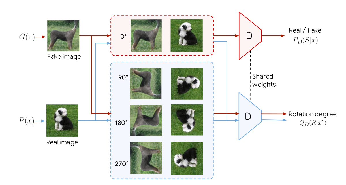
Figure 1: Overview of SSGAN. The original GAN task for the discriminator is kept the same, with the discriminator seeing only upright image to solve this task. However, the discriminator now has an additional task of classifying 1 of 4 rotations of incoming real/fake images.

The key idea of SSGAN lies in using one additional objective to regularize GAN training, on top of having the conventional GAN training objective. This additional objective is the self-supervised task of having the discriminator predict one of four rotations of given real/fake images.

Why is predicting rotations a self-supervised task? The idea is that there are no explicit labels required from humans, and simply performing a transformation on the data is sufficient to obtain a label (or “pseudo-label”) that describes the data. For example, given an image, we can rotate it by 0 degrees, call it class 0, or rotate it by 90 degrees and call it class 1. We can do this for 4 different rotations, so that the set of degrees of rotation \(\mathcal{R} = \{0^\circ, 90^\circ, 180^\circ, 270^\circ\}\) gives classes \(0\) to \(3\) respectively (note the zero-indexing). This is unlike in datasets like ImageNet, where humans are required to explicitly label if an image represents a cat or a dog. Here, our classes are arbitrarily designed, but individually correspond to one of 4 rotations (e.g. class 3 would describe a 270 degrees rotated image). Formally, we can represent the losses for the generator (G) and discriminator (D) as such:

\[\mathcal{L}_G = -V(G, D) - \alpha \mathbb{E}_{x\sim P_G} \mathbb{E}_{r \sim \mathcal{R}}[\log Q_D(R=r \vert x^r)]\]

\[\mathcal{L}_D = V(G, D) - \beta \mathbb{E}_{x\sim P_{\text data}} \mathbb{E}_{r \sim \mathcal{R}}[\log Q_D(R=r \vert x^r)]\]

where V represents the GAN value function, \(P_G\) represents the generated image distribution, \(x^r\) represents a rotated image, and \(Q_D\) represents the classification predictive distribution of a given rotated image, which we can obtain using an additional fully-connected (FC) layer.

Understanding the above 2 equations from the paper is important, since it explicitly tells us that only the rotation loss from the fake images is applied for the generator, and correspondingly, only the rotation loss from real images is applied for the discriminator. Intuitively, this makes sense since we do not want the discriminator to be penalised for fake images that not look realistic, and the generator should strive to produce images that look natural enough to be rotated in a way that is easy for the auxiliary classifier to solve.

While this method of predicting rotations is simple, it has seen excellent performance in representation learning (Gidaris 2018). The insight from SSGAN is that one could use this self-supervised objective to alleviate a key problem in GANs: catastrophic forgetting of the discriminator. The paper presents further insights into this, for which the reader is highly encouraged to read.

However, to simplify the above expression into a form we can implement, we can express for some optimal discriminator \(\hat{D}\) and optimal generator \(\hat {G}\).

\[\mathcal{L}_G = \mathcal{L}_{\text{GAN}}(G, \hat{D}) + \alpha \mathcal{L}_{SS}\]

\[\mathcal{L}_D = \mathcal{L}_{\text{GAN}}(\hat{G}, D) + \beta \mathcal{L}_{SS}\]

where \(\mathcal{L}_{\text{GAN}}\) is simply the hinge loss for GANs, and \(\mathcal{L}_{SS}\) is the self-supervised loss for the rotation, which we can implement as a standard cross entropy loss. In Mimicry, the hinge loss is already implemented, so we only need to implement the self-supervised loss. Here, \(\alpha\) and \(\beta\) refer to the loss scales for the self-supervised loss.

Implementing Models

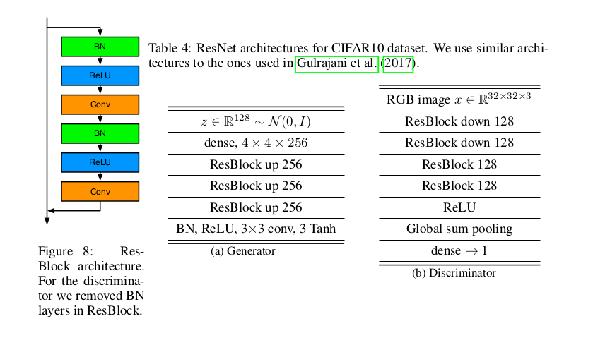
Figure 2: Residual backbone networks for generator and discriminator.

Firstly, we construct the models based on the residual network backbone architectures, which have been frequently used in recent state-of-the-art GANs. SSGAN similarly does this and follows the architecture in Miyato et al, where Spectral Normalization GAN (SNGAN) was introduced. which we similarly adopt. Figure 2 illustrates this particular set of backbone architectures. Specifically, we know from Figure 2 the key variables are:

• nz=128: The initial noise vector dimension is 128.
• ngf=256: The generator feature map size is 256.
• ndf=128: The discriminator feature map size is 128.
• bottom_width=4: The initial spatial resolution for progressively increasing resolution at the generator is 4.

Having done so, we are only left to implement the specific ways to train our GAN. We import several tools we’ll need later in advance:

import torch
import torch.nn as nn
import torch.nn.functional as F
import torch.optim as optim

import numpy as np

import torch_mimicry as mmc
from torch_mimicry.nets import gan
from torch_mimicry.modules import SNLinear
from torch_mimicry.modules import GBlock, DBlock, DBlockOptimized

Discriminator

Now, we define an SSGANDiscriminator class that inherits from an abstract base class BaseDiscriminator, which is a basic definition of an unconditional GAN discriminator in Mimicry. This class requires the discriminator feature map size ndf and a loss_type argument, which we can simply set it as the hinge loss.

class SSGANDiscriminator(gan.BaseDiscriminator):
    def __init__(self, ndf=128, loss_type='hinge', **kwargs):
        super().__init__(ndf=ndf, loss_type=loss_type, **kwargs)

Now, we define some variables that we’ll need to use later. We know that the number of rotations is 4, so we have 4 classes. For scaling the SS loss, this is the \(\beta\) variable in the paper which is set to 1.0.

class SSGANDiscriminator(gan.BaseDiscriminator):
    def __init__(self, ndf=128, loss_type='hinge', **kwargs):
        super().__init__(ndf=ndf, loss_type=loss_type, **kwargs)
        self.num_classes = 4
        self.ss_loss_scale = 1.0

To define the layers, we can simply follow Figure 2 and use the residual blocks. For the discriminator, we need to use DBlock and DBlockOptimized. These residual blocks are similar, except that DBlockOptimized is the first residual block that is always used. This naming convention and design follows closely to the original SNGAN implementation. By default, we have spectral normalization enabled for all residual blocks, although we can set spectral_norm=False to disable it. Since SSGAN uses spectral normalization, we can safely ignore this argument and follow Figure 2’s table for defining the layers:

class SSGANDiscriminator(gan.BaseDiscriminator):
    def __init__(self, ndf=128, loss_type='hinge', **kwargs):
        super().__init__(ndf=ndf, loss_type=loss_type, **kwargs)
        self.num_classes = 4
        self.ss_loss_scale = 1.0

        # Build layers
        self.block1 = DBlockOptimized(3, self.ndf)
        self.block2 = DBlock(self.ndf, self.ndf, downsample=True)
        self.block3 = DBlock(self.ndf, self.ndf, downsample=False)
        self.block4 = DBlock(self.ndf, self.ndf, downsample=False)
        self.l5 = SNLinear(self.ndf, 1)
        self.activation = nn.ReLU(True)

        nn.init.xavier_uniform_(self.l5.weight.data, 1.0)

However, we need to define an additional fully-connected layer for our rotation classification, which in total gives the full model definition:

class SSGANDiscriminator(gan.BaseDiscriminator):
    def __init__(self, ndf=128, loss_type='hinge', **kwargs):
        super().__init__(ndf=ndf, loss_type=loss_type, **kwargs)
        self.num_classes = 4
        self.ss_loss_scale = 1.0

        # Build layers
        self.block1 = DBlockOptimized(3, self.ndf)
        self.block2 = DBlock(self.ndf, self.ndf, downsample=True)
        self.block3 = DBlock(self.ndf, self.ndf, downsample=False)
        self.block4 = DBlock(self.ndf, self.ndf, downsample=False)
        self.l5 = SNLinear(self.ndf, 1)
        self.activation = nn.ReLU(True)

        nn.init.xavier_uniform_(self.l5.weight.data, 1.0)

        # Rotation class prediction layer
        self.l_y = SNLinear(self.ndf, self.num_classes)
        nn.init.xavier_uniform_(self.l_y.weight.data, 1.0)

Following Figure 2, we can define the feedforward function of the paper in a similar way as defining a regular PyTorch model, except that we now need to output our rotation class logits:

def forward(self, x):
    """
    Feedforwards a batch of real/fake images and produces a batch of GAN logits,
    and rotation classes.
    """
    h = x
    h = self.block1(h)
    h = self.block2(h)
    h = self.block3(h)
    h = self.block4(h)
    h = self.activation(h)

    # Global sum pooling
    h = torch.sum(h, dim=(2, 3))
    output = self.l5(h)

    # Produce the class output logits
    output_classes = self.l_y(h)

    return output, output_classes

Now, we need to define several functions to rotate our images. In SSGAN, the image batch is split into 4 quarters, and each quarter is rotated with a unique direction. For example, for a batch size of 64, the images 1-16 are 0 degrees rotated, images 17-32 are 90 degrees rotated, and so on. We define a function that can easily rotate a given image:

def _rot_tensor(self, image, deg):
    """
    Rotation for pytorch tensors using rotation matrix. Takes in a tensor of (C, H, W shape).
    """
    if deg == 90:
        return image.transpose(1, 2).flip(1)

    elif deg == 180:
        return image.flip(1).flip(2)

    elif deg == 270:
        return image.transpose(1, 2).flip(2)

    elif deg == 0:
        return image

    else:
        raise NotImplementedError(
            "Function only supports 90,180,270,0 degree rotation.")

To rotate an entire batch of images, we can define a function, which rotates the image and gives us the corresponding rotated labels back. These labels are our “pseudo-labels” that we have arbitrarily created for the model.

def _rotate_batch(self, images):
    """
    Rotate a quarter batch of images in each of 4 directions.
    """
    N, C, H, W = images.shape
    choices = [(i, i * 4 // N) for i in range(N)]

    # Collect rotated images and labels
    ret = []
    ret_labels = []
    degrees = [0, 90, 180, 270]
    for i in range(N):
        idx, rot_label = choices[i]

        # Rotate images
        image = self._rot_tensor(images[idx],
                                 deg=degrees[rot_label])  # (C, H, W) shape
        image = torch.unsqueeze(image, 0)  # (1, C, H, W) shape

        # Get labels accordingly
        label = torch.from_numpy(np.array(rot_label))  # Zero dimension
        label = torch.unsqueeze(label, 0)

        ret.append(image)
        ret_labels.append(label)

    # Concatenate images and labels to (N, C, H, W) and (N, ) shape respectively.
    ret = torch.cat(ret, dim=0)
    ret_labels = torch.cat(ret_labels, dim=0).to(ret.device)

    return ret, ret_labels

To compute the SS loss from a given batch of upright (non-rotated) images, we can define the following function that rotates this batch of image, obtain the classification logits for computing the SS loss, and scaling the loss correspondingly:

def compute_SS_loss(self, images, scale):
    """
    Function to compute SS loss.
    """
    # Rotate images and produce labels here.
    images_rot, class_labels = self.rotate_batch(
        images=images)

    # Compute SS loss
    _, output_classes = self.forward(images_rot)

    err_SS = F.cross_entropy(
        input=output_classes,
        target=class_labels)

    # Scale SS loss
    err_SS = scale * err_SS

    return err_SS

Finally, a crucial step is to define the train_step function to analyze how these components can produce a training step for the discriminator. We define the train_step function that requires 4 key components:

• real_batch: The input batch of images and labels,
• netG: The input generator for generating fake images.
• optD: The optimizer for the discriminator update.
• log_data: A MetricLog object that we can use to collect our data in the pipeline.

where device and global_step are optional arguments which we can ignore if we are not using them. Doing so, we can produce the GAN loss in a way similar to training a DCGAN, where we first produce the logits. For real images, this can be obtained from our real_batch argument, but for fake images, we can simply call the in-built generate_images.

def train_step(self,
               real_batch,
               netG,
               optD,
               log_data,
               device=None,
               global_step=None,
               **kwargs):
    """
    Train step function for discriminator.
    """
    self.zero_grad()

    # Produce real images
    real_images, _ = real_batch
    batch_size = real_images.shape[0]  # Match batch sizes for last iter

    # Produce fake images
    fake_images = netG.generate_images(num_images=batch_size,
                                       device=device).detach()

    # Compute real and fake logits for gan loss
    output_real, _ = self.forward(real_images)
    output_fake, _ = self.forward(fake_images)

Now, we want to compute our losses, where we can use our functions compute_gan_loss (in-built from our base class), and the function we defined compute_ss_loss:

# Compute GAN loss, upright images only.
errD = self.compute_gan_loss(output_real=output_real,
                             output_fake=output_fake)

# Compute SS loss, rotates the images. -- only for real images!
errD_SS = self.compute_ss_loss(images=real_images,
                               scale=self.ss_loss_scale)

# Backprop and update gradients
errD_total = errD + errD_SS
errD_total.backward()
optD.step()

We can produce extra metrics for logging our progress, such as the probabilities of the discriminator thinking a real/fake image is real. We can add these information with log_data using its add_metric function, giving it a name and group to belong to. Here, group is optional but allows you to group together losses such as errD and errG to be on the same diagram in TensorBoard.

# Compute probabilities
D_x, D_Gz = self.compute_probs(output_real=output_real,
                               output_fake=output_fake)

# Log statistics for D
log_data.add_metric('errD', errD, group='loss')
log_data.add_metric('errD_SS', errD_SS, group='loss_SS')
log_data.add_metric('D(x)', D_x, group='prob')
log_data.add_metric('D(G(z))', D_Gz, group='prob')

return log_data

Our final train step function for the discriminator looks is this function returning log_data as before, since log_data acts like a “message” that is being passed down the training pipeline to collect more information:

def train_step(self,
               real_batch,
               netG,
               optD,
               log_data,
               device=None,
               global_step=None,
               **kwargs):
    """
    Train step function for discriminator.
    """
    self.zero_grad()

    # Produce real images
    real_images, _ = real_batch
    batch_size = real_images.shape[0]  # Match batch sizes for last iter

    # Produce fake images
    fake_images = netG.generate_images(num_images=batch_size,
                                       device=device).detach()

    # Compute real and fake logits for gan loss
    output_real, _ = self.forward(real_images)
    output_fake, _ = self.forward(fake_images)

    # Compute GAN loss, upright images only.
    errD = self.compute_gan_loss(output_real=output_real,
                                 output_fake=output_fake)

    # Compute SS loss, rotates the images. -- only for real images!
    errD_SS = self.compute_ss_loss(images=real_images,
                                   scale=self.ss_loss_scale)

    # Backprop and update gradients
    errD_total = errD + errD_SS
    errD_total.backward()
    optD.step()

    # Compute probabilities
    D_x, D_Gz = self.compute_probs(output_real=output_real,
                                   output_fake=output_fake)

    # Log statistics for D once out of loop
    log_data.add_metric('errD', errD, group='loss')
    log_data.add_metric('errD_SS', errD_SS, group='loss_SS')
    log_data.add_metric('D(x)', D_x, group='prob')
    log_data.add_metric('D(G(z))', D_Gz, group='prob')

    return log_data

Generator

Constructing the generator is a lot simpler, as the structure is similar to SNGAN’s generator except that we now need to consider an additional train step function. Similar to previously, let’s define the generator object by inheriting from the BaseGenerator abstract class and building the layers according to Figure 2:

class SSGANGenerator(gan.BaseGenerator):
    def __init__(self,
                 nz=128,
                 ngf=256,
                 bottom_width=4,
                 loss_type='hinge',
                 **kwargs):
        super().__init__(nz=nz,
                         ngf=ngf,
                         bottom_width=bottom_width,
                         loss_type=loss_type,
                         **kwargs)
        self.ss_loss_scale = 0.2

        # Build the layers
        self.l1 = nn.Linear(self.nz, (self.bottom_width**2) * self.ngf)
        self.block2 = GBlock(self.ngf, self.ngf, upsample=True)
        self.block3 = GBlock(self.ngf, self.ngf, upsample=True)
        self.block4 = GBlock(self.ngf, self.ngf, upsample=True)
        self.b5 = nn.BatchNorm2d(self.ngf)
        self.c5 = nn.Conv2d(ngf, 3, 3, 1, padding=1)
        self.activation = nn.ReLU(True)

        # Initialise the weights
        nn.init.xavier_uniform_(self.l1.weight.data, 1.0)
        nn.init.xavier_uniform_(self.c5.weight.data, 1.0)

Here, we note that ss_loss_scale corresponds to the \(\alpha\) parameter in the paper, which is set to 0.2 for all datasets.

The feedforward function is simply passing some input noise through all these layers, following Figure 2 to use tanh for the activation. This is important since the output images will have values in the range [-1, 1], which is the range we would normalize our images to:

def forward(self, x):
    """
    Feedforward function.
    """
    h = self.l1(x)
    h = h.view(x.shape[0], -1, self.bottom_width, self.bottom_width)
    h = self.block2(h)
    h = self.block3(h)
    h = self.block4(h)
    h = self.b5(h)
    h = self.activation(h)
    h = torch.tanh(self.c5(h))

    return h

For the train_step function, we similarly take in 4 key arguments:

• real_batch: The input batch of images and labels,
• netD: The input discriminator for getting logits (in contrast to defining netG).
• optG: The optimizer for the generator update (in contrast to defining optD).
• log_data: A MetricLog object that we can use to log our data to tensorboard/printing.

We can similarly produce our GAN and SS losses like previously, and update them.

def train_step(self,
               real_batch,
               netD,
               optG,
               log_data,
               device=None,
               global_step=None,
               **kwargs):
    """
    Train step function.
    """
    self.zero_grad()

    # Get only batch size from real batch
    batch_size = real_batch[0].shape[0]

    # Produce fake images and logits
    fake_images = self.generate_images(num_images=batch_size,
                                       device=device)
    output, _ = netD(fake_images)

    # Compute GAN loss, upright images only.
    errG = self.compute_gan_loss(output)

    # Compute SS loss, rotates the images -- fake images only!
    errG_SS = netD.compute_ss_loss(images=fake_images,
                                   scale=self.ss_loss_scale)

    # Backprop and update gradients
    errG_total = errG + errG_SS
    errG_total.backward()
    optG.step()

Now we can use add_metric again, but we want to group our metric to be in the same group as errD and errD_SS, so we can visualize them more nicely in TensorBoard. This is optional, but would be something nice to do.

# Log statistics
log_data.add_metric('errG', errG, group='loss')
log_data.add_metric('errG_SS', errG_SS, group='loss_SS')

We return a log_data object like before, and have our final train_step function looking like:

def train_step(self,
               real_batch,
               netD,
               optG,
               log_data,
               device=None,
               global_step=None,
               **kwargs):
    """
    Train step function.
    """
    self.zero_grad()

    # Get only batch size from real batch
    batch_size = real_batch[0].shape[0]

    # Produce fake images and logits
    fake_images = self.generate_images(num_images=batch_size,
                                       device=device)
    output, _ = netD(fake_images)

    # Compute GAN loss, upright images only.
    errG = self.compute_gan_loss(output)

    # Compute SS loss, rotates the images. -- fake images only!
    errG_SS = netD.compute_ss_loss(images=fake_images,
                                   scale=self.ss_loss_scale)

    # Backprop and update gradients
    errG_total = errG + errG_SS
    errG_total.backward()
    optG.step()

    # Log statistics
    log_data.add_metric('errG', errG, group='loss')
    log_data.add_metric('errG_SS', errG_SS, group='loss_SS')

    return log_data

Training

Once the two models are constructed, training the GAN is as straightforward. we can define the basic parts of our training pipeline: our dataloader, models, and optimizers. We use the Adam optimizer, and note that the beta parameters are chosen to be \((\beta_1, \beta_2) = (0.0, 0.9)\) following the paper, which traditionally have worked well for GAN training. To construct the components of the pipeline:

# Directories
dataset_dir = './datasets'
log_dir = './log/ssgan'

# Data handling objects
dataset = mmc.datasets.load_dataset(root='./datasets', name='cifar10')
dataloader = torch.utils.data.DataLoader(
    dataset, batch_size=64, shuffle=True, num_workers=4)

# Define models and optimizers
device = torch.device('cuda:0' if torch.cuda.is_available() else "cpu")
netG = SSGANGenerator().to(device)
netD = SSGANDiscriminator().to(device)
optD = optim.Adam(netD.parameters(), 2e-4, betas=(0.0, 0.9))
optG = optim.Adam(netG.parameters(), 2e-4, betas=(0.0, 0.9))

Having these components done, we can simply build a Trainer object to build the pipeline and start training!

# Start training
trainer = mmc.training.Trainer(
    netD=netD,
    netG=netG,
    optD=optD,
    optG=optG,
    n_dis=2,
    num_steps=100000,
    dataloader=dataloader,
    log_dir=log_dir)

trainer.train()

Here, we note that n_dis is the number of discriminator update steps per generator update step, which is set to 2 in the paper. The paper further notes that SSGAN is trained for 100K generator steps, which we follow.

Doing so, we can see the following outputs during training:

INFO: [Epoch 1/127][Global Step: 2/100000]
| D(G(z)): 0.9987
| D(x): 0.9992
| errD: 7.7222
| errD_SS: 3.6375
| errG: 2.0727
| errG_SS: 0.9488
| lr_D: 0.0002
| lr_G: 0.0002
| (0.4046 sec/idx)
^CINFO: Saving checkpoints from keyboard interrupt...
INFO: Training Ended.

and one can dynamically stop at any part of the training if required.

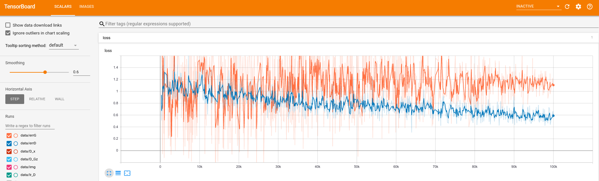
Figure 3: Tensorboard visualizations of smoothened GAN losses.

After 100K training steps, we can visualise our training from Tensorboard with tensorboard --logdir=./log/ssgan, which produces curves as seen in Figure 3.

Internally, a Logger object that is defined within Trainer would also visualise images randomly generated every 500 steps, and also images generated from a fixed set of noise vectors. This has 2 benefits: random images allows us to check the diversity of images continuously, in case there is mode collapse, and fixed random images where we can assess the quality of the images generated continuously. Figures 4 and 5 give some examples.

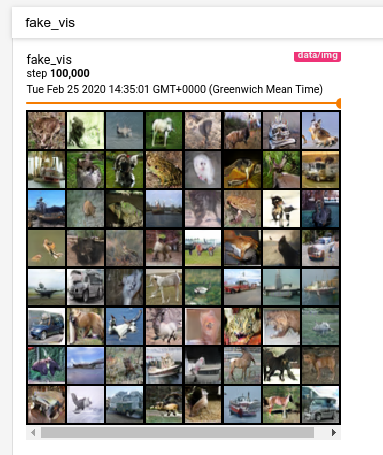
Figure 4: Randomly generated images in TensorBoard for checking diversity.

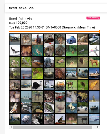
Figure 5: Tensorboard visualisation of randomly generated images from a set of fixed noise vectors, to assess quality of images over training.

However it might be hard to understand the benefit of the second without a concrete example. Fortunately, the Logger object also saves the fixed fake images as png files every 500 steps (configurable), which we can then use to generate a gif! We see this result in Figure 6 – could you observe the gradual formation of certain classes like horses and cars?

Figure 6: GIF output from images generated from a set of fixed noise vector, as saved every 500 steps from the start of training till the end.

Evaluation

When assessing GANs, it is difficult to simply judge how good a GAN is through only a qualitative assessment of images. Several quantitative metrics have been proposed, and one of which is the Fréchet Inception Distance (FID), which is also used in the SSGAN paper. Generally, FID measures the Wasserstein-2 distance between the Inception features, by assuming their distributions take the form of a multivariate Gaussian. These inception features are obtained through using an ImageNet pre-trained Inception model, which is traditionally the one from TensorFlow, as used by the original authors of FID, and similarly by authors of other metrics like Inception Score (IS) and Kernel Inception Distance(KID).

Naturally, changing the pre-trained inception model would cause some differences in the output inception features. Thus, to ensure backwards compatibility of the computed scores, Mimicry adopts the original TensorFlow implementations of all metrics from the authors, without exposing the TensorFlow backend to users.

Doing so, we can simply perform evaluate our FID using

mmc.metrics.evaluate(
    metric='fid',
    log_dir=log_dir,
    netG=netG,
    dataset_name='cifar10',
    num_real_samples=10000,
    num_fake_samples=10000,
    evaluate_step=100000,
    device=device)

By default, we will run 3 times for computing FID, and report the mean and standard deviation of the scores towards the end:

INFO: Loading existing statistics for real images...
INFO: Generated image 1000/10000 [Random Seed 0] (0.0011 sec/idx)
INFO: Generated image 2000/10000 [Random Seed 0] (0.0009 sec/idx)
INFO: Generated image 3000/10000 [Random Seed 0] (0.0009 sec/idx)
INFO: Generated image 4000/10000 [Random Seed 0] (0.0009 sec/idx)
INFO: Generated image 5000/10000 [Random Seed 0] (0.0009 sec/idx)
INFO: Generated image 6000/10000 [Random Seed 0] (0.0009 sec/idx)
INFO: Generated image 7000/10000 [Random Seed 0] (0.0009 sec/idx)
INFO: Generated image 8000/10000 [Random Seed 0] (0.0009 sec/idx)
INFO: Generated image 9000/10000 [Random Seed 0] (0.0009 sec/idx)
INFO: Generated image 10000/10000 [Random Seed 0] (0.0009 sec/idx)
INFO: Computing statistics for fake images...
INFO: Propagated batch 200/200 (0.2466 sec/batch)
INFO: FID (step 100000) [seed 0]: 17.950461181932667
INFO: Computing FID in memory...
...
...
INFO: Generated image 8000/10000 [Random Seed 1] (0.0009 sec/idx)
INFO: Generated image 9000/10000 [Random Seed 1] (0.0009 sec/idx)
INFO: Generated image 10000/10000 [Random Seed 1] (0.0009 sec/idx)
...
...
INFO: FID (step 100000) [seed 1]: 17.46868878132358
...
...
INFO: FID (step 100000) [seed 2]: 17.883670445065718
INFO: FID (step 100000): 17.767606802773987 (± 0.2131184933218733)
INFO: FID Evaluation completed!

where we can cache our existing real image statistics to avoid hefty recomputation, and also compare the generator’s performance with the same set of real image statistics as it trains. We cache our result as a JSON file in the log directory, so we can avoid re-computing the scores at the same global step.

How well did we perform? From the paper, for the exact training hyperparameters, the FID is reported to be 17.88 ± 0.64, whereas we achieved 17.77 ± 0.21 so our result is very close!

Final Code

The overall code required to build this customised GAN can be found here. While we have built the models from scratch as seen above, SSGAN is currently one of the standard implementations available in Mimicry, where you can import mmc.nets.ssgan.SSGANGenerator32 and mmc.nets.ssgan.SSGANDiscriminator32 directly.

Conclusion

Mimicry allows researchers to focus a lot more on the GAN implementation, which as you have experienced, takes up bulk of the work! This reduces the need to re-implement boilerplate code for training and evaluation, so one can focus on the research. For a list of GANs we support, see Reproducibility. For a list of over 70 baseline scores (at the time of this writing), see Baselines.

Feel free to contact me if you’d like to find out more about the work!